How Delhi Buses
Move in 2026
The roads become faster as the evening progresses, but speed is only part of the passenger experience. Six hours of bus GPS reveal slow corridors, uneven service and the limits of a fixed-speed timetable.
Switch the map between peak and late-night conditions. Drag to pan, use the chart toolbar to zoom, and hover for values. Every interactive chart includes a data table and a CSV download.
One evening, observed at ten-second intervals.
The source is the Delhi Government and IIIT-Delhi Open Transit Data vehicle-position feed.
The collection contains approximately 5.1 million positions from 6,065 buses. After trajectory checks, 3,626,697 usable GPS steps remain for speed analysis. The speed field in the feed is zero, so speeds must be calculated from consecutive positions.
The reporting fleet shrinks through the evening.
Figure 01View the data table.
| Input | Coverage and purpose |
|---|---|
| Live vehicle positions | The six-hour feed supplies vehicle, route and trip identifiers, timestamps and coordinates. It supports observed trajectories rather than planned journeys. |
| Archived 2023 GTFS | The archived static feed supplies stops, routes and planned stop times. Duplicate stops are merged into 5,319 locations. |
| Rebuilt 2026 routes | Observed stop passages reconstruct 1,421 live routes because live route identifiers do not directly match the archived timetable. |
| Missing observations | About 6% of polls are empty. The longest consecutive empty-response period is 30 seconds. An empty response is a collection gap, not evidence that every bus stopped operating. |
Vehicle timestamps can precede the time a response was collected. The collection window and the earliest reported vehicle observation are therefore not identical. Raw positions and credentials are not published with this report.
From positions to transport measures.
This is a reproducible batch analysis. It does not require an always-running collector to read the saved results.
- Collect and deduplicate the feed.Python requests retrieves GTFS-Realtime messages. The GTFS bindings decode the protocol buffer. The collector keeps changed observations, and the analysis selects the longest continuous collection period.
- Calculate usable movement.pandas and NumPy order positions by bus and timestamp. Haversine distance and elapsed time supply speed. Stale positions, GPS jumps above 80 km/h, long observation gaps and layovers of at least five minutes are excluded from usable steps.
- Match stops and rebuild routes.The pipeline clusters duplicate archived stops, checks bus direction and detects 483,177 stop passages. Stops are ordered by median time since a trip began, producing route sequences that can be compared with the archive.
- Aggregate road speeds.Positions are grouped into a 110 m Web Mercator grid. Each qualifying cell has at least three observations. Distance and time totals are smoothed separately over neighbouring cells before their ratio is converted to km/h.
- Measure service and arrival times.Stop passages supply travel times and gaps between buses on the same route at the same stop. The model uses distance, route, starting stop, time, prediction horizon and recent speed information.
| Technical layer | Libraries and responsibilities |
|---|---|
| Storage and processing | pandas and NumPy handle transformations. PyArrow stores intermediate tables as Parquet. SciPy supports spatial processing and grid smoothing. |
| Prediction | LightGBM trains the arrival-time regression model. Simple historical and recent-speed baselines make the comparison interpretable. |
| Notebook maps | Matplotlib and contextily produce static maps with Esri basemaps. Those maps remain available in the notebook. |
| Interactive report | Locally bundled Plotly.js renders aggregate grids and charts. Plain HTML, CSS and JavaScript run on GitHub Pages without a backend. The interactive road map needs no external map tiles. |
The network clears after the peak.
The map measures speeds on observed bus corridors. It is not a congestion census of every Delhi road.
Explore the observed roads at two times of the evening.
Figure 02View the data table.
The peak affects a broad area.
About 45% of qualifying road cells are below 15 km/h at the evening peak, compared with about 14% late at night. The busy and quiet windows use the same grid and colour scale.
Coverage changes with the fleet.
Fewer buses report late at night. Each window therefore has its own set of qualifying cells. The change is descriptive, not a controlled comparison of an identical set of roads.
Typical speeds rise, but individual observations vary widely.
Figure 03View the data table.
The median usable-step speed rises from 8.6 km/h in the 18:00 hour to about 25 km/h after 23:00.This is a median of observed GPS-step speeds. The road map instead uses aggregated distance divided by time, so the two measures are not interchangeable.
Short stretches can still absorb several minutes.
Figure 04View the data table.
The slowest qualifying stretch is ISBT Anand Vihar to Maharaj Pur Check Post. Its 264 m straight-line distance takes a median 7.1 minutes, implying 2.2 km/h. Several slow stretches are near terminals or depots, where queueing and entry delays can contribute to the measured time.
Faster roads do not guarantee even service.
A passenger experiences the gap between buses as well as the journey time after boarding.
Observed gaps include both close arrivals and long waits.
Figure 05View the data table.
Compare service frequency with arrival irregularity.
Figure 06View the data table.
Close arrivals are common.
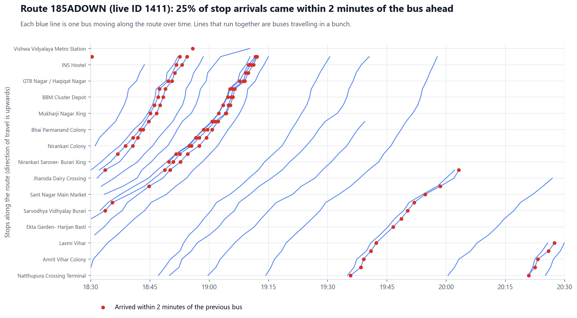
About one in eight of the 315,366 observed gaps is under two minutes. This is evidence of clustered arrivals under the analysis definition, but it does not identify the operational cause of every cluster.
Regularity deserves a separate target.
About 41% of assessed routes have a headway coefficient of variation of at least one. Adding vehicles alone may not resolve uneven spacing. Dispatch and holding decisions would need a separate operational evaluation.
See one route's saved time-space diagram.
Each line follows one bus along route 185A. The marked close arrivals illustrate the citywide definition without replacing the aggregate analysis.
Compare the model against useful baselines.
The task is to predict elapsed time from a stop to each of the next one to ten stops.
The training pipeline creates about 1.3 million arrival examples. LightGBM is compared with a historical median and a bus's own recent speed. Three test designs expose different kinds of generalisation.
The apparent gain depends on the test design.
Figure 07View the data table.
Error grows with the number of stops ahead.
Figure 08View the data table.
The same-hours result is the clearest baseline comparison.
LightGBM reduces mean absolute error from 98.8 to 84.6 seconds, an improvement of about 14%. On unseen routes, the reduction is about 24%, from 151.7 to 115.2 seconds.
The largest gain needs context.
The later-evening improvement is about 42%, but early peak traffic makes the historical baseline a poor guide to late-night conditions. That figure should not be presented as the model's universal benefit.
Distance and the starting stop account for about two-thirds of the model's feature gain. The live speed of buses ahead contributes about 5%, while a bus's own recent speed contributes very little. Feature importance describes this fitted model; it does not establish a causal effect.
The 2023 timetable is context, not a current service promise.
The archive and the live feed are separated by roughly three and a half years.
A constant-speed timetable misses the evening's changing conditions.
Figure 09View the data table.
- The pipeline strongly matches 368 live routes to archived routes by stop sequence. The frequency comparison uses 290 qualifying routes, not all 1,421 rebuilt routes.
- Those qualifying routes show 2,759 observed trips against 2,243 planned trips between 19:00 and 23:00, approximately 23% more. This indicates a difference between snapshots, not proof that service improved across the whole network.
- At least three buses pass 4,636 of the 5,319 clustered archived stop locations, approximately 87%. Locations not passed could reflect changed stops, changed routes or a lack of evening service.
Separate road delay, service spacing and information quality.
They affect passengers differently and require different operational responses.
What the evidence supports.
This evening's observations show substantial speed recovery after the peak, persistent slow stop-to-stop stretches and uneven gaps between buses. A data-driven arrival model improves on simple baselines, but its measured benefit changes with the evaluation design.
What a transport project owner could do next.
- Investigate specific bottlenecks before proposing citywide changes.Use the slow stretches near Anand Vihar, Gazipur and Mahipalpur as candidates for field observation. Distinguish road congestion from depot entry, terminal queueing and stop dwell before selecting an intervention.
- Track service regularity separately from travel speed.Assess close arrivals and long gaps on frequent routes. Any dispatch or holding trial should measure changes in headway variability and passenger waiting, rather than assuming more vehicles automatically create better service.
- Use the model as an evaluated prototype.The same-hours result supports further testing of live arrival estimates. New days, weather conditions, morning peaks and disrupted routes should be held out before deployment decisions are made.
- Improve the reference data.An updated static feed would reduce ambiguity in stop matching, route naming and timetable comparisons. Historical route mismatches should not be treated as failures by today's operator.
What cannot be concluded from this project.
- Six hours on one weekday cannot establish annual reliability, weekend behaviour or a morning-peak pattern.
- The feed does not measure passenger loads, unmet demand, crowding or actual passenger waiting time. These are priorities for operational assessment, not measured outcomes here.
- Straight-line stop distances can understate road distance. Matching to archived stops can miss newly introduced locations.
- No intervention was tested, so the analysis cannot quantify the benefit of a new bus lane, different dispatch policy or timetable revision.
Sources and reproducibility.
- Vehicle data comes from Delhi Open Transit Data, operated by the Department of Transport, Government of NCT of Delhi, and IIIT-Delhi, under the portal's data terms.
- The 2023 GTFS archive is documented in the data guide. The interactive map is drawn from aggregate GPS grids, without external basemap requests.
- The notebook, model summary and processing scripts preserve the analysis. Static notebook basemaps credit Esri, HERE, Garmin and OpenStreetMap contributors.